Process Mining - Part 2

This is a continuation from Part 1 on the topic of process mining.

One of bupaR’s coolest features is the ability to animate a process. The animation represents the movement of cases through the processes, based on the timing data. Check this out:

animate_process(elc)

In the following sections, I’ll list a quick rundown of a few more features from bupaR. Really, this is just scratching the surface of what bupaR and process mining can provide - I encourage you if you’re interested in this topic to check out bupaR and start a journey of your own.

We can add a measure of performance in terms of timing to the process map. Here I’ve added median minutes for the activities, with a view of relative frequencies (replacing the absolute frequencies we saw earlier). We can see clearly now that the movement from “Upload Documents” to “Process Documents” is the heaviest consumer of the timing at over 78 minutes:

elc %>%
  process_map(type_nodes = frequency("relative_case"), performance(median, "mins", color_scale = "Purples"))

How is the workload distributed amongst the team ? Let’s have a look at just that Settlement activity and see:

el %>%
  filter(objectTypeDesc == 'Settlement') %>%
  resource_involvement("resource") %>%
  plot()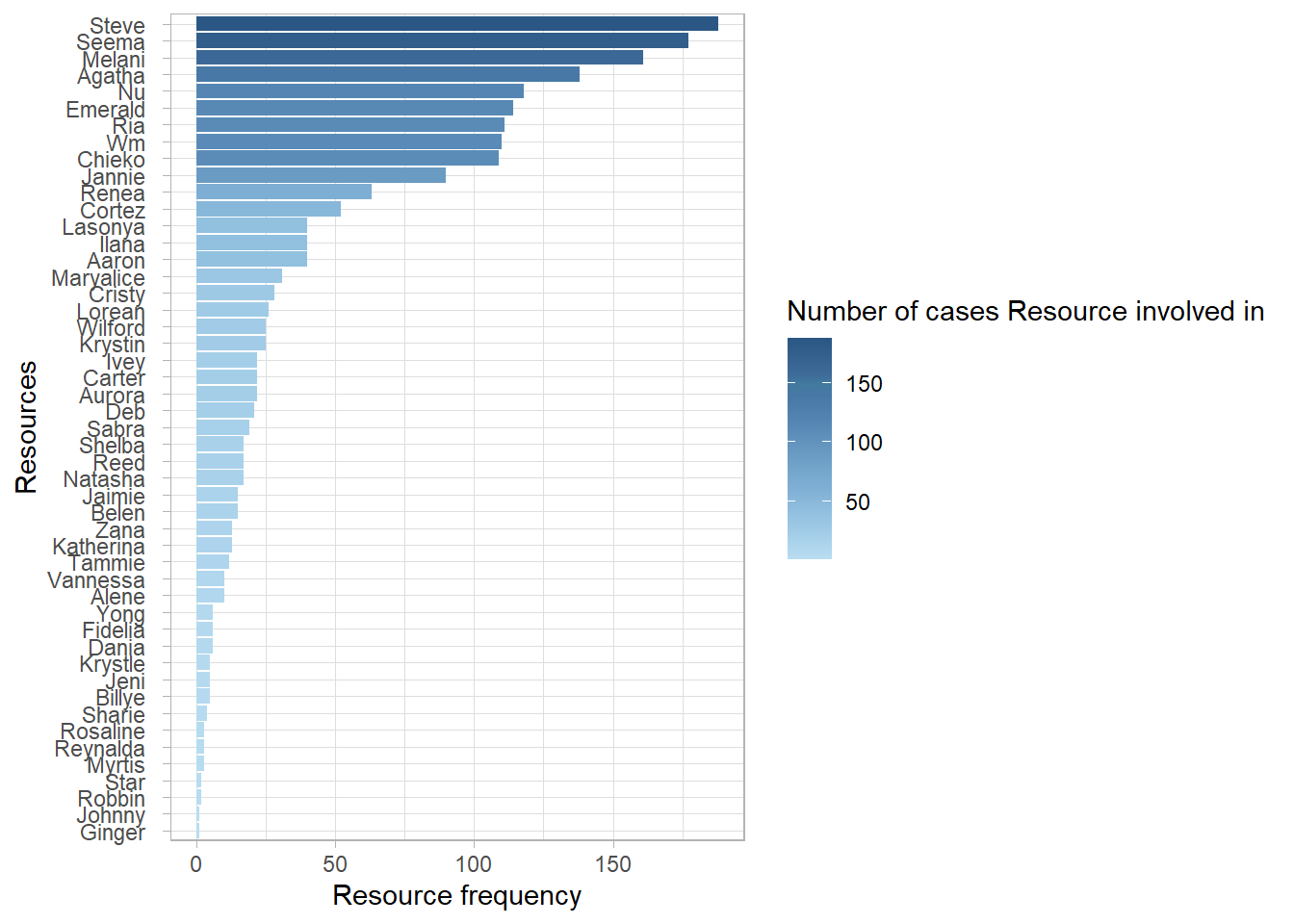

In bupaR, “traces” show the different activity sequences that occur. It may be of interest to view both the most common and least common sequences. Here we will narrow down again to just that Settlement activity to see how the statuses move in different sequences within there:

el %>%
  filter(objectTypeDesc == 'Settlement') %>%
  trace_explorer(coverage = 0.5)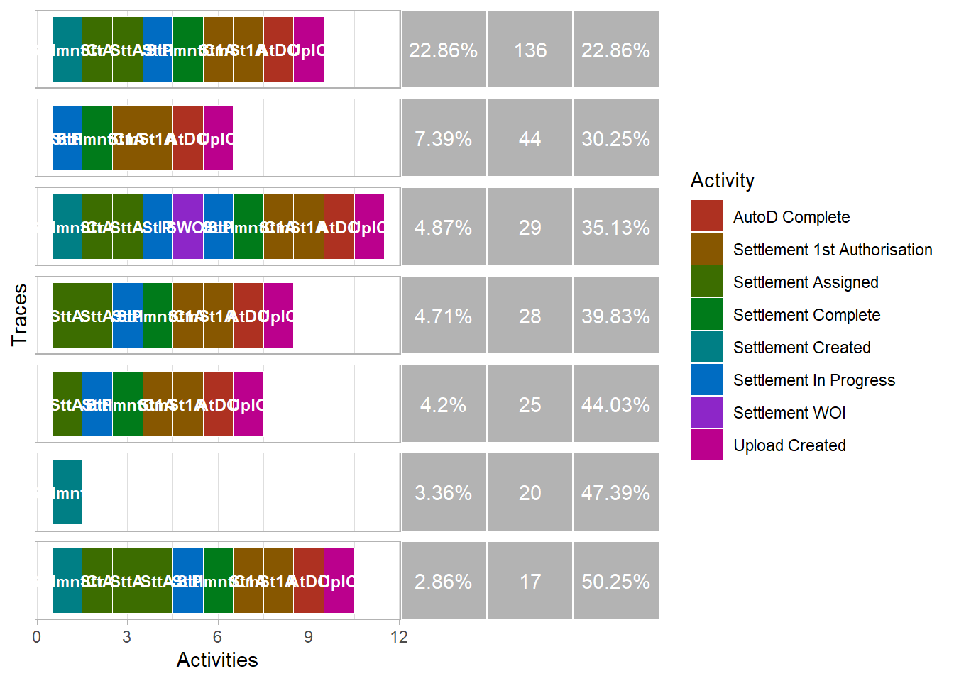

Thank you for reading !